API Documentation¶

superphot.fit module¶

class superphot.fit.LogUniform(name, *args, **kwargs)[source]¶

Bases: pymc3.distributions.continuous.BoundedContinuous

Continuous log-uniform log-likelihood.

The pdf of this distribution is

\[f(x \mid lower, upper) = \frac{1}{[\log(upper)-\log(lower)]x}\]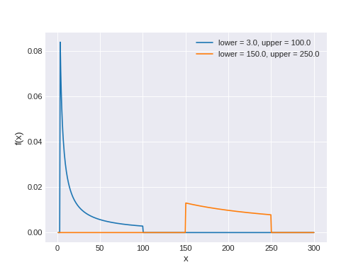

Support	$x \in [lower, upper]$
Mean	$\dfrac{upper - lower}{\log(upper) - \log(lower)}$

Parameters

lowerfloat: Lower limit.
upperfloat: Upper limit.

logp(value)[source]¶

Calculate log-probability of LogUniform distribution at specified value.

Parameters

valuenumeric: Value for which log-probability is calculated.

Returns

TensorVariable

random(point=None, size=None)[source]¶

Draw random values from LogUniform distribution.

Parameters

pointdict, optional: Dict of variable values on which random values are to be conditioned (uses default point if not specified).
sizeint, optional: Desired size of random sample (returns one sample if not specified).

Returns

array

superphot.fit.cut_outliers(t, nsigma)[source]¶

Make an Astropy table containing only data that is below the cut off threshold.

Parameters

tastropy.table.Table: Astropy table containing the light curve data.
nsigmafloat: Determines at what value (flux < nsigma * mad_std) to cut outlier data points.

Returns

t_cutastropy.table.Table: Astropy table containing only data that is below the cut off threshold.

superphot.fit.diagnostics(obs, trace, parameters, filename='.', show=False)[source]¶

Make some diagnostic plots for the PyMC3 fitting.

Parameters

obsastropy.table.Table: Observed light curve data in a single filter.
tracepymc3.MultiTrace: Trace object that is the result of the PyMC3 fit.
parameterslist: List of Theano variables in the PyMC3 model.
filenamestr, optional: Directory in which to save the output plots and summary. Not used if show=True.
showbool, optional: If True, show the plots instead of saving them.

superphot.fit.flux_model(t, A, beta, gamma, t_0, tau_rise, tau_fall)[source]¶

Calculate the flux given amplitude, plateau slope, plateau duration, reference epoch, rise time, and fall time using theano.switch. Parameters.type = TensorType(float64, scalar).

Parameters

t1-D numpy array: Time.
ATensorVariable: Amplitude of the light curve.
betaTensorVariable: Light curve slope during the plateau, normalized by the amplitude.
gammaTensorVariable: The duration of the plateau after the light curve peaks.
t_0TransformedRV: Reference epoch.
tau_riseTensorVariable: Exponential rise time to peak.
tau_fallTensorVariable: Exponential decay time after the plateau ends.

Returns

flux_modelsymbolic Tensor: The predicted flux from the given model.

superphot.fit.make_new_priors(traces, parameters, res=100)[source]¶

For each parameter, combine the posteriors for the four filters and use that as the new prior.

Parameters

tracesdict: Dictionary of MultiTrace objects for each filter.
parameterslist: List of Theano variables for which to combine the posteriors. (Only names of the parameters are used.)
resint, optional: Number of points to sample the KDE for the new priors.

Returns

x_priorslist: List of Numpy arrays containing the x-values of the new priors.
y_priorslist: List of Numpy arrays containing the y-values of the new priors.
old_posteriorslist: List of dictionaries containing the y-values of the old posteriors for each filter.

superphot.fit.plot_final_fits(t, traces1, traces2, parameters, outfile=None)[source]¶

Make a four-panel plot showing sample light curves from each of the two fitting iterations compared to observations.

Parameters

tastropy.table.Table: Astropy table containing the observed light curve.
traces1, traces2dict: Dictionaries of the trace objects (for each filter) from which to generate the model light curves.
parameterslist: List of Theano variables in the PyMC3 model.
outfilestr, optional: Filename to which to save the plot. If None, display the plot instead of saving it.

Returns

figmatplotlib.figure.Figure: Figure object for the plot (can be added to a multipage PDF).

superphot.fit.plot_model_lcs(obs, trace, parameters, size=100, ax=None, fltr=None, ls=None, phase_min=- 50.0, phase_max=180.0)[source]¶

Plot sample light curves from a fit compared to the observations.

Parameters

obsastropy.table.Table: Astropy table containing the observed light curve in a single filter.
tracepymc3.MultiTrace: PyMC3 trace object containing values for the fit parameters.
parameterslist: List of Theano variables in the PyMC3 model.
sizeint, optional: Number of draws from the posterior to plot. Default: 100.
axmatplotlib.axes.Axes, optional: Axes object on which to plot the light curves. If None, create new Axes.
fltrstr, optional: Filter these data were observed in. Only used to label and color the plot.
lsstr, optional: Line style for the model light curves. Default: solid line.
phase_min, phase_maxfloat, optional: Time range over which to plot the light curves.

superphot.fit.plot_priors(x_priors, y_priors, old_posteriors, parameters, saveto=None)[source]¶

Overplot the old priors, the old posteriors in each filter, and the new priors for each parameter.

Parameters

x_priorslist: List of Numpy arrays containing the x-values of the new priors.
y_priorslist: List of Numpy arrays containing the y-values of the new priors.
old_posteriorslist: List of dictionaries containing the y-values of the old posteriors for each filter.
parameterslist: List of Theano variables for which to combine the posteriors.
savetostr, optional: Filename to which to save the plot. If None, display the plot instead of saving it.

superphot.fit.produce_lc(time, trace, align_to_t0=False)[source]¶

Load the stored PyMC3 traces and produce model light curves from the parameters.

Parameters

timenumpy.array: Range of times (in days, with respect to PEAKMJD) over which the model should be calculated.
tracenumpy.array: PyMC3 trace stored as an array, with parameters as the last dimension.
align_to_t0bool, optional: Interpret time as days with respect to t_0 instead of PEAKMJD.

Returns

lcnumpy.array: Model light curves. Time is the last dimension.

superphot.fit.read_light_curve(filename)[source]¶

Read light curve data from a text file as an Astropy table. SNANA files are recognized.

Parameters

filenamestr: Path to light curve data file.

Returns

tastropy.table.Table: Table of light curve data.

superphot.fit.sample_or_load_trace(model, trace_file, force=False, iterations=10000, walkers=25, tuning=25000, cores=1)[source]¶

Run a Metropolis Hastings MCMC for the given model with a certain number iterations, burn in (tuning), and walkers.

If the MCMC has already been run, read and return the existing trace (unless force=True).

Parameters

modelpymc3.Model: PyMC3 model object for the input data.
trace_filestr: Path where the trace will be stored. If this path exists, load the trace from there instead.
forcebool, optional: Resample the model even if trace_file already exists.
iterationsint, optional: The number of iterations after tuning.
walkersint, optional: The number of cores and walkers used.
tuningint, optional: The number of iterations used for tuning.
coresint, optional: The number of walkers to run in parallel. Default: 1.

Returns

tracepymc3.MultiTrace: The PyMC3 trace object for the MCMC run.

superphot.fit.select_event_data(t, phase_min=- 50.0, phase_max=180.0, nsigma=None)[source]¶

Select data only from the period containing the peak flux, with outliers cut.

Parameters

tastropy.table.Table: Astropy table containing the light curve data.
phase_min, phase_maxfloat, optional: Include only points within [phase_min, phase_max) days of SEARCH_PEAKMJD.
nsigmafloat, optional: Determines at what value (flux < nsigma * mad_std) to reject outlier data points. Default: no rejection.

Returns

t_eventastropy.table.Table: Table containing the reduced light curve data from the period containing the peak flux.

superphot.fit.setup_model1(obs, max_flux=None)[source]¶

Set up the PyMC3 model object, which contains the priors and the likelihood.

Parameters

obsastropy.table.Table: Astropy table containing the light curve data.
max_fluxfloat, optional: The maximum flux observed in any filter. The amplitude prior is 100 * max_flux. If None, the maximum flux in the input table is used, even though it does not contain all the filters.

Returns

modelpymc3.Model: PyMC3 model object for the input data. Use this to run the MCMC.

superphot.fit.setup_model2(obs, parameters, x_priors, y_priors)[source]¶

Set up a PyMC3 model for observations in a given filter using the given priors and parameter names.

Parameters

obsastropy.table.Table: Astropy table containing the light curve data.
parameterslist: List of Theano variables for which to create new parameters. (Only names of the parameters are used.)
x_priorslist: List of Numpy arrays containing the x-values of the priors.
y_priorslist: List of Numpy arrays containing the y-values of the priors.

Returns

modelpymc3.Model: PyMC3 model object for the input data. Use this to run the MCMC.

superphot.fit.two_iteration_mcmc(light_curve, outfile, filters=None, force=False, force_second=False, do_diagnostics=True, iterations=10000, walkers=25, tuning=25000)[source]¶

Fit the model to the observed light curve. Then combine the posteriors for each filter and use that as the new prior for a second iteration of fitting.

Parameters

light_curveastropy.table.Table: Astropy table containing the observed light curve.
outfilestr: Path where the trace will be stored. This should include a blank field ({{}}) that will be replaced with the iteration number and filter name. Diagnostic plots will also be saved according to this pattern.
filtersstr, optional: Light curve filters to fit. Default: all filters in light_curve.
forcebool, optional: Redo the fit (both iterations) even if results are already stored in outfile. Default: False.
force_secondbool, optional: Redo only the second iteration of the fit, even if the results are already stored in outfile. Default: False.
do_diagnosticsbool, optional: Produce and save some diagnostic plots. Default: True.
iterationsint, optional: The number of iterations after tuning.
walkersint, optional: The number of cores and walkers used.
tuningint, optional: The number of iterations used for tuning.

Returns

traces1, traces2dict: Dictionaries of the PyMC3 trace objects for each filter for the first and second fitting iterations.
parameterslist: List of Theano variables in the PyMC3 model.

superphot.extract module¶

superphot.extract.compile_data_table(filename)[source]¶

superphot.extract.compile_parameters(stored_models, filters, ndraws=10, random_state=None)[source]¶

Read the saved PyMC3 traces and compile an array of fit parameters for each transient. Save to a Numpy file.

Parameters

stored_modelsstr: Look in this directory for PyMC3 trace data and sample the posterior to produce model LCs.
filtersiterable: Filters for which to compile parameters. These should be the last characters of the subdirectories in which the traces are stored.
ndrawsint, optional: Number of random draws from the MCMC posterior. Default: 10.
random_stateint, optional: Seed for the random number generator, which is used to sample the posterior. Use for reproducibility.

superphot.extract.extract_features(t, zero_point=27.5, use_median=False, use_pca=True, stored_pcas=None, save_pca_to=None, save_reconstruction_to=None)[source]¶

Extract features for a table of model light curves: the peak absolute magnitudes and principal components of the light curves in each filter.

Parameters

tastropy.table.Table: Table containing the ‘params’/’median_params’, ‘redshift’, and ‘MWEBV’ of each transient to be classified.
zero_pointfloat, optional: Zero point to be used for calculating the peak absolute magnitudes. Default: 27.5 mag.
use_medianbool, optional: Use the median parameters to produce the light curves instead of the multiple draws from the posterior.
use_pcabool, optional: Use the peak absolute magnitudes and principal components of the light curve as the features (default). Otherwise, use the model parameters directly.
stored_pcasstr, optional: Path to pickled PCA objects. Default: create and fit new PCA objects.
save_pca_tostr, optional: Plot and save the principal components to this file. Default: skip this step.
save_reconstruction_tostr, optional: Plot and save the reconstructed light curves to this file (slow). Default: skip this step.

Returns

t_goodastropy.table.Table: Slice of the input table with a ‘features’ column added. Rows with any bad features are excluded.

superphot.extract.flux_to_luminosity(row, R_filter)[source]¶

Return the flux-to-luminosity conversion factor for the transient in a given row of a data table.

Parameters

rowastropy.table.row.Row: Astropy table row for a given transient, containing columns ‘MWEBV’ and ‘redshift’.
R_filterlist: Ratios of A_filter to row[‘MWEBV’] for each of the filters used. This determines the length of the output.

Returns

flux2lumnumpy.ndarray: Array of flux-to-luminosity conversion factors for each filter.

superphot.extract.get_principal_components(light_curves, n_components=6, whiten=True)[source]¶

Run a principal component analysis on a set of light curves for each filter.

Parameters

light_curvesarray-like: An array of model light curves to be used for fitting the PCA.
n_componentsint, optional: The number of principal components to calculate. Default: 6.
whitenbool, optional: Whiten the input data before calculating the principal components. Default: True.

Returns

pcaslist: A list of the PCA objects for each filter.

superphot.extract.load_trace(tracefile, filters)[source]¶

Read the stored PyMC3 traces into a 3-D array with shape (nsteps, nfilters, nparams).

Parameters

tracefilestr: Directory where the traces are stored. Should contain an asterisk (*) to be replaced by elements of filters.
filtersiterable: Filters for which to load traces. If one or more filters are not found, the posteriors of the remaining filters will be combined and used in place of the missing ones.

Returns

trace_valuesnumpy.array: PyMC3 trace stored as 3-D array with shape (nsteps, nfilters, nparams).

superphot.extract.plot_feature_correlation(data_table, saveto=None)[source]¶

Plot a matrix of the Spearman rank correlation coefficients between each pair of features.

Parameters

data_tableastropy.table.Table: Astropy table containing a ‘features’ column. Must also have ‘featnames’ and ‘filters’ in data_table.meta.
savetostr, optional: Filename to which to save the plot. Default: show instead of saving.

superphot.extract.plot_pca_reconstruction(models, reconstructed, time=None, coefficients=None, filters=None, titles=None, saveto='pca_reconstruction.pdf')[source]¶

Plot comparisons between the model light curves and the light curves reconstructed from the PCA for each transient. These are saved as a multipage PDF.

Parameters

modelsarray-like: A 3-D array of model light curves with shape (ntransients, nfilters, ntimes)
reconstructedarray-like: A 3-D array of reconstructed light curves with shape (ntransients, nfilters, ntimes)
timearray-like, optional: A 1-D array of times that correspond to the last axis of models. Default: x-axis will run from 0 to ntimes.
coefficientsarray-like, optional: A 3-D array of the principal component coefficients with shape (ntransients, nfilters, ncomponents). If given, the coefficients will be printed at the top right of each plot.
filtersiterable, optional: Names of the filters corresponding to the PCA objects. Only used for coloring the lines.
titlesiterable, optional: Titles for each plot.
savetostr, optional: Filename for the output file. Default: pca_reconstruction.pdf.

superphot.extract.plot_principal_components(pcas, time=None, filters=None, saveto='principal_components.pdf')[source]¶

Plot the principal components being used to extract features from the model light curves.

Parameters

pcaslist: List of the PCA objects for each filter, after fitting.
timearray-like, optional: Times (x-values) to plot the principal components against.
filtersiterable, optional: Names of the filters corresponding to the PCA objects. Only used for coloring and labeling the lines.
savetostr, optional: Filename to which to save the plot. Default: principal_components.pdf.

superphot.extract.project_onto_principal_components(light_curves, pcas)[source]¶

Project a set of light curves onto their principal components for each filter.

Parameters

light_curvesarray-like: An array of model light curves to be projected onto the principal components.
pcaslist: A list of the PCA objects for each filter.

Returns

coefficientsnumpy.ndarray: An array of the coefficients on the principal components.
reconstructednumpy.ndarray: An reconstruction of the light curves from their principal components.

superphot.extract.save_data(t, basename)[source]¶

superphot.extract.select_good_events(t, data)[source]¶

Select only events with finite data for all draws. Returns the table and data for only these events.

Parameters

tastropy.table.Table: Original data table. Must have t.meta[‘ndraws’] to indicate now many draws it contains for each event.
dataarray-like, shape=(nfilt, len(t), …): Numpy array containing the data upon which finiteness will be judged.

Returns

t_goodastropy.table.Table: Data table containing only the good events.
good_dataarray-like: Numpy array containing only the data for good events.

superphot.classify module¶

class superphot.classify.MultivariateGaussian(sampling_strategy='all', random_state=None)[source]¶

Bases: imblearn.over_sampling.base.BaseOverSampler

Class to perform over-sampling using a multivariate Gaussian (numpy.random.multivariate_normal).

Parameters

sampling_strategyfloat, str, dict, callable or int, default=’auto’

Sampling information to resample the data set.

When float, it corresponds to the desired ratio of the number of samples in the minority class over the number of samples in the majority class after resampling. Therefore, the ratio is expressed as $\alpha_{os} = N_{rm} / N_{M}$ where $N_{rm}$ is the number of samples in the minority class after resampling and $N_{M}$ is the number of samples in the majority class.

Warning

float is only available for binary classification. An error is raised for multi-class classification.
When str, specify the class targeted by the resampling. The number of samples in the different classes will be equalized. Possible choices are:

'minority': resample only the minority class;

'not minority': resample all classes but the minority class;

'not majority': resample all classes but the majority class;

'all': resample all classes;

'auto': equivalent to 'not majority'.
When dict, the keys correspond to the targeted classes. The values correspond to the desired number of samples for each targeted class.
When callable, function taking y and returns a dict. The keys correspond to the targeted classes. The values correspond to the desired number of samples for each class.
When int, it corresponds to the total number of samples in each class (including the real samples). Can be used to oversample even the majority class. If sampling_strategy is smaller than the existing size of a class, that class will not be oversampled and the classes may not be balanced.

random_stateint, RandomState instance, default=None

Control the randomization of the algorithm.

If int, random_state is the seed used by the random number generator;
If RandomState instance, random_state is the random number generator;
If None, the random number generator is the RandomState instance used by np.random.

more_samples(n_samples)[source]¶: Draw more samples from the same distribution of an already fitted sampler.

superphot.classify.aggregate_probabilities(table)[source]¶

Average the classification probabilities for a given supernova across the multiple model light curves.

Parameters

tableastropy.table.Table: Astropy table containing the metadata for a supernova and the classification probabilities (‘probabilities’)

Returns

resultsastropy.table.Table: Astropy table containing the supernova metadata and average classification probabilities for each supernova

superphot.classify.bar_plot(vresults, tresults, saveto=None)[source]¶

Make a stacked bar plot showing the class breakdown in the training set compared to the test set.

Parameters

vresultsastropy.table.Table: Astropy table containing the training data. Must have a ‘type’ column and a ‘prediction’ column.
tresultsastropy.table.Table: Astropy table containing the test data. Must have a ‘prediction’ column.
savetostr, optional: Save the plot to this filename. If None, the plot is displayed and not saved.

superphot.classify.calc_metrics(results, param_set, save=False)[source]¶

Calculate completeness, purity, accuracy, and F1 score for a table of validation results.

The metrics are returned in a dictionary and saved in a json file.

Parameters

resultsastropy.table.Table: Astropy table containing the results. Must have columns ‘type’ and ‘prediction’.
param_setdict: A dictionary containing metadata to store along with the metrics.
savebool, optional: If True, save the results to a json file in addition to returning the results. Default: False

Returns

param_setdict: A dictionary containing the input metadata and the calculated metrics.

superphot.classify.classify(pipeline, test_data, aggregate=True)[source]¶

Use a trained classification pipeline to classify test_data.

Parameters

pipelineimblearn.pipeline.Pipeline: The full classification pipeline, including rescaling, resampling, and classification.
test_dataastropy.table.Table: Astropy table containing the test data. Must have a ‘features’ column.
aggregatebool, optional: If True (default), average the probabilities for a given supernova across the multiple model light curves.

Returns

resultsastropy.table.Table: Astropy table containing the supernova metadata and classification probabilities for each supernova

superphot.classify.cumhist(data, reverse=False, mark=None, ax=None, **kwargs)[source]¶

Plot a cumulative histogram of data, optionally with certain indices marked with an x.

Parameters

dataarray-like: Data to include in the histogram
reversebool, optional: If False (default), the histogram increases with increasing data. If True, it decreases with increasing data
markarray-like, optional: An array of indices to mark with an x
axmatplotlib.pyplot.axes, optional: Axis on which to plot the confusion matrix. Default: current axis.
kwargsdict, optional: Keyword arguments to be passed to matplotlib.pyplot.step

Returns

plist: The list of matplotlib.lines.Line2D objects returned by matplotlib.pyplot.step

superphot.classify.load_results(filename)[source]¶

superphot.classify.make_confusion_matrix(results, classes=None, p_min=0.0, saveto=None, purity=False, binary=False, title=None)[source]¶

Given a data table with classification probabilities, calculate and plot the confusion matrix.

Parameters

resultsastropy.table.Table: Astropy table containing the supernova metadata and classification probabilities (column name = ‘probabilities’)
classesarray-like, optional: Labels corresponding to the ‘probabilities’ column. If None, use the sorted entries in the ‘type’ column.
p_minfloat, optional: Minimum confidence to be included in the confusion matrix. Default: include all samples.
savetostr, optional: Save the plot to this filename. If None, the plot is displayed and not saved.
puritybool, optional: If False (default), aggregate by row (true label). If True, aggregate by column (predicted label).
binarybool, optional: If True, plot a SNIa vs non-SNIa (CCSN) binary confusion matrix.
titlestr, optional: A title for the plot. If the plot is big enough, statistics ($N$, $A$, $F_1$) are appended in parentheses. Default: ‘Completeness’ or ‘Purity’ depending on purity.

superphot.classify.mean_axis0(x, axis=0)[source]¶: Equivalent to the numpy.mean function but with axis=0 by default.

superphot.classify.plot_confusion_matrix(confusion_matrix, classes, cmap='Blues', purity=False, title='', xlabel='Photometric Classification', ylabel='Spectroscopic Classification', ax=None)[source]¶

Plot a confusion matrix with each cell labeled by its fraction and absolute number.

Based on tutorial: https://scikit-learn.org/stable/auto_examples/model_selection/plot_confusion_matrix.html

Parameters

confusion_matrixarray-like: The confusion matrix as a square array of integers.
classeslist: List of class labels for the axes of the confusion matrix.
cmapstr, optional: Name of a Matplotlib colormap to color the matrix.
puritybool, optional: If False (default), aggregate by row (spec. class). If True, aggregate by column (phot. class).
titlestr, optional: Text to go above the plot. Default: no title.
xlabel, ylabelstr, optional: Labels for the x- and y-axes. Default: “Spectroscopic Classification” and “Photometric Classification”.
axmatplotlib.pyplot.axes, optional: Axis on which to plot the confusion matrix. Default: new axis.

superphot.classify.plot_feature_importance(pipeline, train_data, width=0.8, nsamples=1000, saveto=None)[source]¶

Plot a bar chart of feature importance using mean decrease in impurity, with permutation importances overplotted.

Mean decrease in impurity is assumed to be stored in pipeline.feature_importances_. If the classifier does not have this attribute (e.g., SVM, MLP), only permutation importance is calculated.

Parameters

pipelinesklearn.pipeline.Pipeline or imblearn.pipeline.Pipeline: The trained pipeline for which to plot feature importances. Steps should be named ‘classifier’ and ‘sampler’.
train_dataastropy.table.Table: Data table containing ‘features’ and ‘type’ for training when calculating permutation importances. Must also include ‘featnames’ and ‘filters’ in train_data.meta.
widthfloat, optional: Total width of the bars in units of the separation between bars. Default: 0.8.
nsamplesint, optional: Number of samples to draw for the fake validation data set. Default: 1000.
savetostr, optional: Filename to which to save the plot. Default: show instead of saving.

superphot.classify.plot_metrics_by_number(validation, xval='confidence', classes=None, saveto=None)[source]¶

Plot completeness, purity, accuracy, F1 score, and fractions remaining as a function of confidence threshold.

Parameters

validationastropy.table.Table: Astropy table containing the results. Must have columns ‘type’, ‘prediction’, ‘probabilities’, and ‘confidence’.
xvalstr, optional: Table column to use as the horizontal axis of the plot. Default: ‘confidence’.
classesarray-like, optional: The classes for which to calculate completeness and purity. Default: all classes in the ‘type’ column.
savetostr, optional: Save the plot to this filename. If None, the plot is displayed and not saved.

superphot.classify.plot_results_by_number(results, xval='confidence', class_kwd='prediction', title=None, saveto=None)[source]¶

Plot cumulative histograms of the results for each class against a specified table column.

If results contains the column ‘correct’, incorrect classifications will be marked with an x.

Parameters

resultsastropy.table.Table: Table of classification results. Must contain columns ‘type’/’prediction’ and the column specified by xval.
xvalstr, optional: Table column to use as the horizontal axis of the histogram. Default: ‘confidence’.
class_kwdstr, optional: Table column to use as the class grouping. Default: ‘prediction’.
titlestr, optional: Title for the plot. Default: “Training/Test Set, Grouped by {class_kwd}”, where the first word is determined by the presence of the column ‘correct’ in results.
savetostr, optional: Save the plot to this filename. If None, the plot is displayed and not saved.

superphot.classify.train_classifier(pipeline, train_data)[source]¶

Train a classification pipeline on test_data.

Parameters

pipelineimblearn.pipeline.Pipeline: The full classification pipeline, including rescaling, resampling, and classification.
train_dataastropy.table.Table: Astropy table containing the test data. Must have a ‘features’ and a ‘type’ column.

superphot.classify.validate_classifier(pipeline, train_data, test_data=None, aggregate=True)[source]¶

Validate the performance of a machine-learning classifier using leave-one-out cross-validation.

Parameters

pipelineimblearn.pipeline.Pipeline: The full classification pipeline, including rescaling, resampling, and classification.
train_dataastropy.table.Table: Astropy table containing the training data. Must have a ‘features’ column and a ‘type’ column.
test_dataastropy.table.Table, optional: Astropy table containing the test data. Must have a ‘features’ column to which to apply the trained classifier. If None, use the training data itself for validation.
aggregatebool, optional: If True (default), average the probabilities for a given supernova across the multiple model light curves.

Returns

resultsastropy.table.Table: Astropy table containing the supernova metadata and classification probabilities for each supernova

superphot.classify.write_results(test_data, classes, filename, max_lines=None, latex=False, latex_title='Classification Results', latex_label='tab:results')[source]¶

Write the classification results to a text file.

Parameters

test_dataastropy.table.Table: Astropy table containing the supernova metadata and the classification probabilities (‘probabilities’).
classeslist: The labels that correspond to the columns in ‘probabilities’
filenamestr: Name of the output file
max_linesint, optional: Maximum number of table rows to write to the file
latexbool, optional: If False (default), write in the Astropy ‘ascii.fixed_width_two_line’ format. If True, write in the Astropy ‘ascii.aastex’ format and add fancy table headers, etc.
latex_titlestr, optional: Table caption if written in AASTeX format. Default: ‘Classification Results’
latex_labelstr, optional: LaTeX label if written in AASTeX format. Default: ‘tab:results’

superphot.optimize module¶

class superphot.optimize.ParameterOptimizer(pipeline, train_data, validation_data)[source]¶

Bases: object

Class containing the pipeline and data sets for hyperparameter optimization

Parameters

pipelinesklearn.pipeline.Pipeline or imblearn.pipeline.Pipeline: The full classification pipeline, including rescaling, resampling, and classification.
validation_dataastropy.table.Table: Astropy table containing the validation data. Must have a ‘features’ column.
train_dataastropy.table.Table: Astropy table containing the training data. Must have a ‘features’ column and a ‘type’ column.

Attributes

pipelinesklearn.pipeline.Pipeline or imblearn.pipeline.Pipeline: The full classification pipeline, including rescaling, resampling, and classification.
validation_dataastropy.table.Table: Astropy table containing the validation data. Must have a ‘features’ column.
train_dataastropy.table.Table: Astropy table containing the training data. Must have a ‘features’ column and a ‘type’ column.

test_hyperparams(param_set)[source]¶

Validates the pipeline for a set of hyperparameters.

Measures F1 score and accuracy, as well as completeness and purity for each class.

Parameters

param_setdict: A dictionary containing keywords that match the parameters of pipeline and values to which to set them.

Returns

param_setdict: The input param_set with the metrics added to the dictionary. These are also saved to a JSON file.

superphot.optimize.plot_hyperparameters_3d(t, ccols, xcol, ycol, zcol, cmap=None, cmin=None, cmax=None, figtitle='')[source]¶

Plot 3D scatter plots of the metrics against the hyperparameters.

Parameters

tastropy.table.Table: Table of results from test_hyperparameters.
ccolslist: List of columns to plot as metrics.
xcol, ycol, zcolstr: Columns to plot on the x-, y-, and z-axes of the scatter plots.
cmapstr, optional: Name of the colormap to use to color the values in ccols.
cmin, cmaxfloat, optional: Data limits corresponding to the minimum and maximum colors in cmap.
figtitlestr, optional: Title text for the entire multipanel figure.

superphot.optimize.plot_hyperparameters_with_diff(t, dcol=None, xcol=None, ycol=None, zcol=None, saveto=None, **criteria)[source]¶

Plot the metrics for one value of dcol and the difference in the metrics for the second value of dcol.

Parameters

tastropy.table.Table: Table of results from test_hyperparameters.
dcolstr, optional: Column to plot as a difference. Default: alphabetically first column starting with ‘classifier’
xcol, ycol, zcolstr, optional: Columns to plot on the x-, y-, and z-axes of the scatter plots. Default: alphabetically 2nd-4th columns starting wtih ‘classifier’.
savetostr, optional: Save the plot to this filename. If None, the plot is displayed and not saved.
criteriadict, optional: Plot only a subset of the data that matches these keyword-value pairs, and add these criteria to the title. If any keywords do not correspond to table columns, all rows are assumed to match.

superphot.optimize.titlecase(x)[source]¶: Capitalize the first letter of each word in a string (where words are separated by whitespace).

superphot.util module¶

superphot.util.load_data(meta_file, data_file=None)[source]¶

Read input from a text file (the metadata table) and a Numpy file (the features) and return as an Astropy table.

Parameters

meta_filestr: Filename of the input metadata table. Must in an ASCII format readable by Astropy.
data_filestr, optional: Filename where the features are saved. Must be in Numpy binary format. If None, replace the extension of meta_file with .npz.

Returns

data_tableastropy.table.Table: Table containing the metadata along with a ‘features’ column.

superphot.util.plot_histograms(data_table, colname, class_kwd='type', var_kwd=None, row_kwd=None, saveto=None)[source]¶

Plot a grid of histograms of the column colname of data_table, grouped by the column groupby.

Parameters

data_tableastropy.table.Table: Data table containing the columns colname and groupby for each supernova.
colnamestr: Column name of data_table to plot (e.g., ‘params’ or ‘features’).
class_kwdstr, optional: Column name of data_table to group by before plotting (e.g., ‘type’ or ‘prediction’). Default: ‘type’.
var_kwdstr, optional: Keyword in data_table.meta containing the parameter names to list on the x-axes. Default: no labels.
row_kwdstr, optional: Keyword in data_table.meta containing labels for the leftmost y-axes.
savetostr, optional: Filename to which to save the plot. Default: display the plot instead of saving it.

superphot.util.subplots_layout(n)[source]¶

Calculate the number of rows and columns for a multi-panel plot, staying as close to a square as possible.

Parameters

nint: The number of subplots required.

Returns

nrows, ncolsint: The number of rows and columns in the layout.